- Explain artificial neurons with a comparison to biological neurons
- Implement logic gates with Perceptron
- Describe the meaning of Perceptron
- Discuss Sigmoid units and Sigmoid activation function in Neural Network
- Describe ReLU and Softmax Activation Functions
- Explain Hyperbolic Tangent Activation Function
Let’s begin with understanding what is artificial neuron.
Biological Neuron
A human brain has billions of neurons. Neurons are interconnected nerve cells in the human brain that are involved in processing and transmitting chemical and electrical signals. Dendrites are branches that receive information from other neurons.
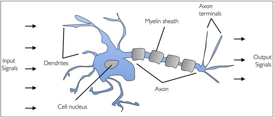
Cell nucleus or Soma processes the information received from dendrites. Axon is a cable that is used by neurons to send information. Synapse is the connection between an axon and other neuron dendrites.
Let us discuss the rise of artificial neurons in the next section.
Rise of Artificial Neurons (Based on Biological Neuron)
Researchers Warren McCullock and Walter Pitts published their first concept of simplified brain cell in 1943. This was called McCullock-Pitts (MCP) neuron. They described such a nerve cell as a simple logic gate with binary outputs.
Multiple signals arrive at the dendrites and are then integrated into the cell body, and, if the accumulated signal exceeds a certain threshold, an output signal is generated that will be passed on by the axon. In the next section, let us talk about the artificial neuron.
What is Artificial Neuron
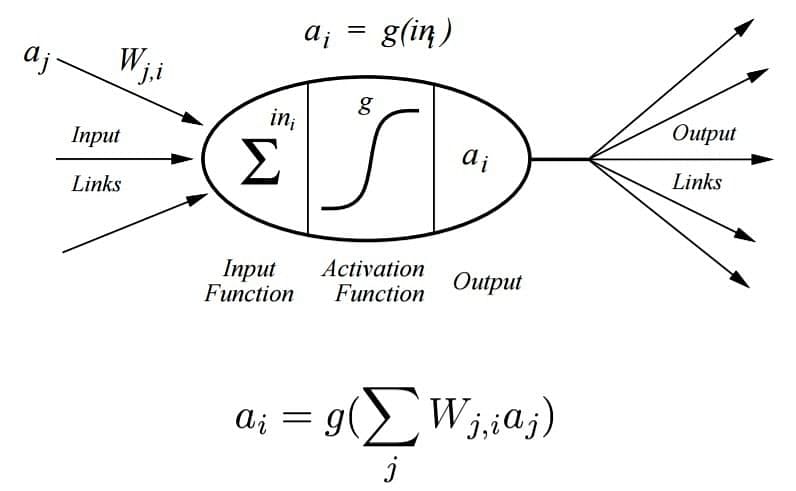
An artificial neuron is a mathematical function based on a model of biological neurons, where each neuron takes inputs, weighs them separately, sums them up and passes this sum through a nonlinear function to produce output.
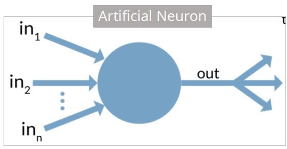
In the next section, let us compare the biological neuron with the artificial neuron.
Biological Neuron vs. Artificial Neuron
The biological neuron is analogous to artificial neurons in the following terms:
Biological Neuron | Artificial Neuron |
Cell Nucleus (Soma) | Node |
Dendrites | Input |
Synapse | Weights or interconnections |
Axon | Output |
Artificial Neuron at a Glance
The artificial neuron has the following characteristics:
- A neuron is a mathematical function modeled on the working of biological neurons
- It is an elementary unit in an artificial neural network
- One or more inputs are separately weighted
- Inputs are summed and passed through a nonlinear function to produce output
- Every neuron holds an internal state called activation signal
- Each connection link carries information about the input signal
- Every neuron is connected to another neuron via connection link
In the next section, let us talk about perceptrons.
Perceptron
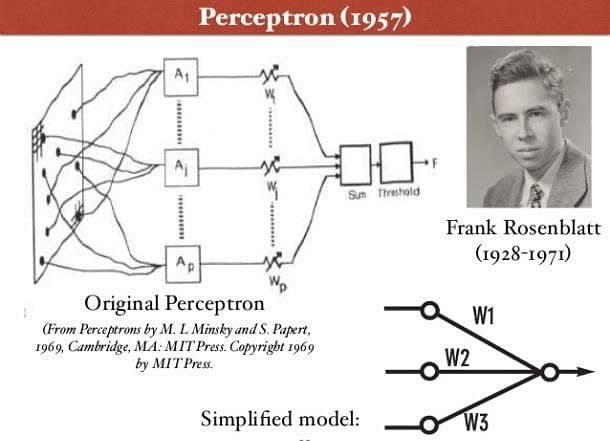
Perceptron was introduced by Frank Rosenblatt in 1957. He proposed a Perceptron learning rule based on the original MCP neuron. A Perceptron is an algorithm for supervised learning of binary classifiers. This algorithm enables neurons to learn and processes elements in the training set one at a time.
There are two types of Perceptrons: Single layer and Multilayer.
- Single layer - Single layer perceptrons can learn only linearly separable patterns
- Multilayer - Multilayer perceptrons or feedforward neural networks with two or more layers have the greater processing power
The Perceptron algorithm learns the weights for the input signals in order to draw a linear decision boundary.
This enables you to distinguish between the two linearly separable classes +1 and -1.
Note: Supervised Learning is a type of Machine Learning used to learn models from labeled training data. It enables output prediction for future or unseen data. Let us focus on the Perceptron Learning Rule in the next section.
Perceptron Learning Rule
Perceptron Learning Rule states that the algorithm would automatically learn the optimal weight coefficients. The input features are then multiplied with these weights to determine if a neuron fires or not.

The Perceptron receives multiple input signals, and if the sum of the input signals exceeds a certain threshold, it either outputs a signal or does not return an output. In the context of supervised learning and classification, this can then be used to predict the class of a sample.
Next up, let us focus on the perceptron function.
Perceptron Function
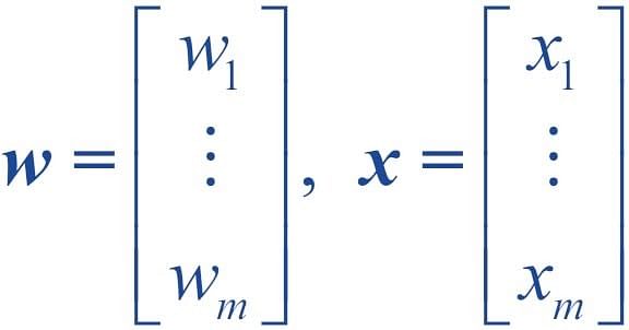
Perceptron is a function that maps its input “x,” which is multiplied with the learned weight coefficient; an output value ”f(x)”is generated.
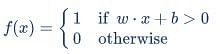
In the equation given above:
- “w” = vector of real-valued weights
- “b” = bias (an element that adjusts the boundary away from origin without any dependence on the input value)
- “x” = vector of input x values

- “m” = number of inputs to the Perceptron
The output can be represented as “1” or “0.” It can also be represented as “1” or “-1” depending on which activation function is used.
Let us learn the inputs of a perceptron in the next section.
Inputs of a Perceptron
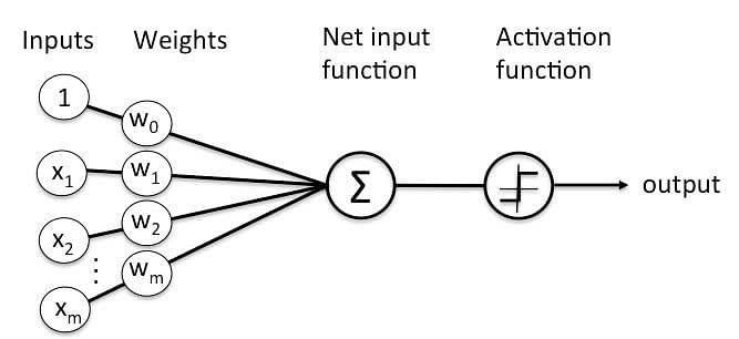
A Perceptron accepts inputs, moderates them with certain weight values, then applies the transformation function to output the final result. The image below shows a Perceptron with a Boolean output.
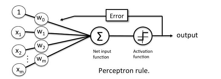
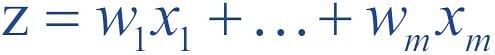
A Boolean output is based on inputs such as salaried, married, age, past credit profile, etc. It has only two values: Yes and No or True and False. The summation function “∑” multiplies all inputs of “x” by weights “w” and then adds them up as follows:
In the next section, let us discuss the activation functions of perceptrons.
Activation Functions of Perceptron
The activation function applies a step rule (convert the numerical output into +1 or -1) to check if the output of the weighting function is greater than zero or not.
For example:
If ∑ wixi> 0 => then final output “o” = 1 (issue bank loan)
Else, final output “o” = -1 (deny bank loan)
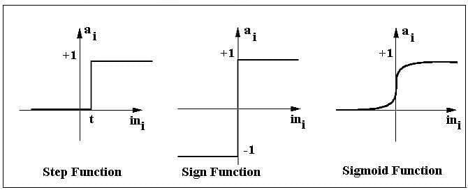
Step function gets triggered above a certain value of the neuron output; else it outputs zero. Sign Function outputs +1 or -1 depending on whether neuron output is greater than zero or not. Sigmoid is the S-curve and outputs a value between 0 and 1.
Output of Perceptron
Perceptron with a Boolean output:
Inputs: x1…xn
Output: o(x1….xn)
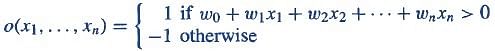
Weights: wi=> contribution of input xi to the Perceptron output;
w0=> bias or threshold
If ∑w.x > 0, output is +1, else -1. The neuron gets triggered only when weighted input reaches a certain threshold value.
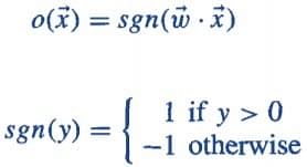
An output of +1 specifies that the neuron is triggered. An output of -1 specifies that the neuron did not get triggered.
“sgn” stands for sign function with output +1 or -1.
Error in Perceptron
In the Perceptron Learning Rule, the predicted output is compared with the known output. If it does not match, the error is propagated backward to allow weight adjustment to happen.
Let us discuss the decision function of Perceptron in the next section.
Perceptron: Decision Function
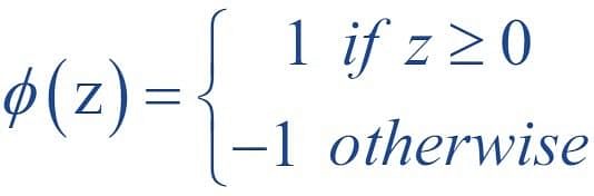
A decision function φ(z) of Perceptron is defined to take a linear combination of x and w vectors.
The value z in the decision function is given by:
The decision function is +1 if z is greater than a threshold θ, and it is -1 otherwise.
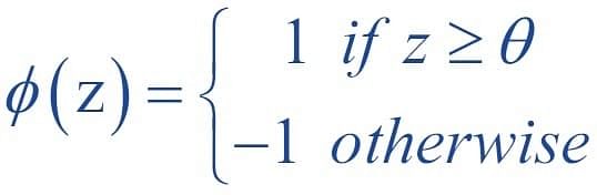
This is the Perceptron algorithm.
Bias Unit
For simplicity, the threshold θ can be brought to the left and represented as w0x0, where w0= -θ and x0= 1.

The value w0 is called the bias unit.
The decision function then becomes:
Output:
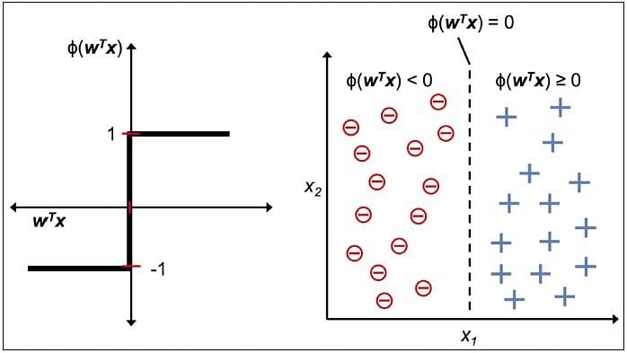
The figure shows how the decision function squashes wTx to either +1 or -1 and how it can be used to discriminate between two linearly separable classes.
Perceptron at a Glance
Perceptron has the following characteristics:
- Perceptron is an algorithm for Supervised Learning of single layer binary linear classifiers.
- Optimal weight coefficients are automatically learned.
- Weights are multiplied with the input features and decision is made if the neuron is fired or not.
- Activation function applies a step rule to check if the output of the weighting function is greater than zero.
- Linear decision boundary is drawn enabling the distinction between the two linearly separable classes +1 and -1.
- If the sum of the input signals exceeds a certain threshold, it outputs a signal; otherwise, there is no output.
Types of activation functions include the sign, step, and sigmoid functions.
Implement Logic Gates with Perceptron
Perceptron - Classifier Hyperplane
The Perceptron learning rule converges if the two classes can be separated by the linear hyperplane. However, if the classes cannot be separated perfectly by a linear classifier, it could give rise to errors.
As discussed in the previous topic, the classifier boundary for a binary output in a Perceptron is represented by the equation given below:
The diagram above shows the decision surface represented by a two-input Perceptron.
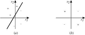
Observation:
- In Fig(a) above, examples can be clearly separated into positive and negative values; hence, they are linearly separable. This can include logic gates like AND, OR, NOR, NAND.
- Fig (b) shows examples that are not linearly separable (as in an XOR gate).
- Diagram (a) is a set of training examples and the decision surface of a Perceptron that classifies them correctly.
- Diagram (b) is a set of training examples that are not linearly separable, that is, they cannot be correctly classified by any straight line.
- X1 and X2 are the Perceptron inputs.
In the next section, let us talk about logic gates.
What is Logic Gate?
Logic gates are the building blocks of a digital system, especially neural networks. In short, they are the electronic circuits that help in addition, choice, negation, and combination to form complex circuits. Using the logic gates, Neural Networks can learn on their own without you having to manually code the logic. Most logic gates have two inputs and one output.
Each terminal has one of the two binary conditions, low (0) or high (1), represented by different voltage levels. The logic state of a terminal changes based on how the circuit processes data.
Based on this logic, logic gates can be categorized into seven types:
- AND
- NAND
- OR
- NOR
- NOT
- XOR
- XNOR
Implementing Basic Logic Gates With Perceptron
The logic gates that can be implemented with Perceptron are discussed below.
1. AND
If the two inputs are TRUE (+1), the output of Perceptron is positive, which amounts to TRUE.
This is the desired behavior of an AND gate.
x1= 1 (TRUE), x2= 1 (TRUE)
w0 = -.8, w1 = 0.5, w2 = 0.5
=> o(x1, x2) => -.8 + 0.5*1 + 0.5*1 = 0.2 > 0
2. OR
If either of the two inputs are TRUE (+1), the output of Perceptron is positive, which amounts to TRUE.
This is the desired behavior of an OR gate.
x1 = 1 (TRUE), x2 = 0 (FALSE)
w0 = -.3, w1 = 0.5, w2 = 0.5
=> o(x1, x2) => -.3 + 0.5*1 + 0.5*0 = 0.2 > 0
3. XOR
A XOR gate, also called as Exclusive OR gate, has two inputs and one output.
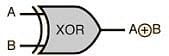
The gate returns a TRUE as the output if and ONLY if one of the input states is true.
XOR Truth Table
Input | Output | |
A | B | |
0 | 0 | 0 |
0 | 1 | 1 |
1 | 0 | 1 |
1 | 1 | 0 |
XOR Gate with Neural Networks
Unlike the AND and OR gate, an XOR gate requires an intermediate hidden layer for preliminary transformation in order to achieve the logic of an XOR gate.
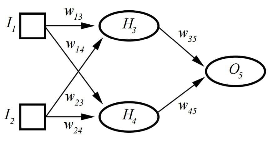
An XOR gate assigns weights so that XOR conditions are met. It cannot be implemented with a single layer Perceptron and requires Multi-layer Perceptron or MLP.
H represents the hidden layer, which allows XOR implementation.
I1, I2, H3, H4, O5are 0 (FALSE) or 1 (TRUE)
t3= threshold for H3; t4= threshold for H4; t5= threshold for O5
H3= sigmoid (I1*w13+ I2*w23–t3); H4= sigmoid (I1*w14+ I2*w24–t4)
O5= sigmoid (H3*w35+ H4*w45–t5);
Next up, let us learn more about the Sigmoid activation function! Which is very important.
Sigmoid Activation Function
The diagram below shows a Perceptron with sigmoid activation function. Sigmoid is one of the most popular activation functions.
A Sigmoid Function is a mathematical function with a Sigmoid Curve (“S” Curve). It is a special case of the logistic function and is defined by the function given below:
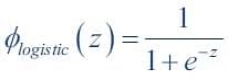
Here, value of z is:
Sigmoid Curve
The curve of the Sigmoid function called “S Curve” is shown here.
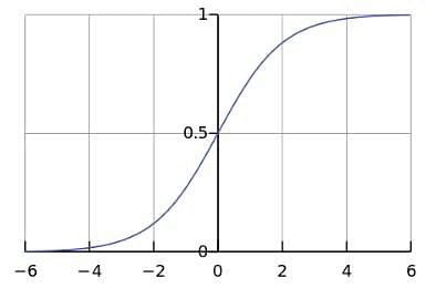
This is called a logistic sigmoid and leads to a probability of the value between 0 and 1.
This is useful as an activation function when one is interested in probability mapping rather than precise values of input parameter t.
The sigmoid output is close to zero for highly negative input. This can be a problem in neural network training and can lead to slow learning and the model getting trapped in local minima during training. Hence, hyperbolic tangent is more preferable as an activation function in hidden layers of a neural network.
Sigmoid Logic for Sample Data
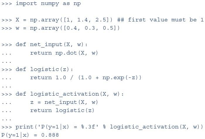
Output
The Perceptron output is 0.888, which indicates the probability of output y being a 1.
If the sigmoid outputs a value greater than 0.5, the output is marked as TRUE. Since the output here is 0.888, the final output is marked as TRUE.
In the next section, let us focus on the rectifier and softplus functions.
Rectifier and Softplus Functions
Apart from Sigmoid and Sign activation functions seen earlier, other common activation functions are ReLU and Softplus. They eliminate negative units as an output of max function will output 0 for all units 0 or less.
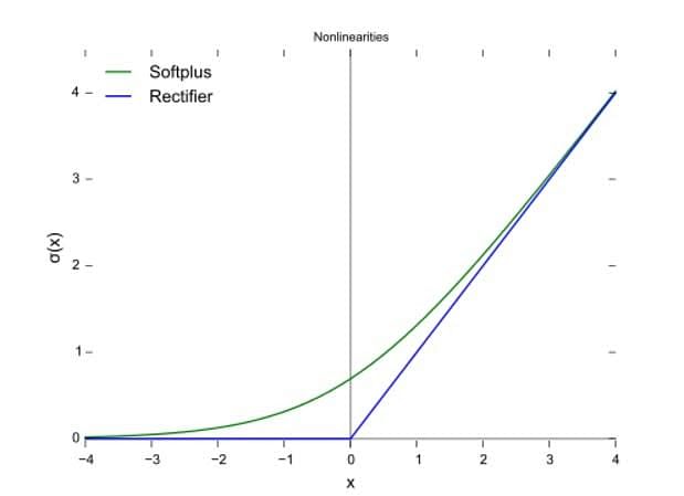
A rectifier or ReLU (Rectified Linear Unit) is a commonly used activation function. This function allows one to eliminate negative units in an ANN. This is the most popular activation function used in deep neural networks.
- A smooth approximation to the rectifier is the Softplus function.
- The derivative of Softplus is the logistic or sigmoid function.
In the next section, let us discuss the advantages of ReLu function.
Advantages of ReLu Functions
The advantages of ReLu function are as follows:
- Allows faster and more effective training of deep neural architectures on large and complex datasets
- Sparse activation of only about 50% of units in a neural network (as negative units are eliminated)
- More plausible or one-sided, compared to anti-symmetry of tanh
- Efficient gradient propagation, which means no vanishing or exploding gradient problems
- Efficient computation with the only comparison, addition, or multiplication
- Scales well
- Non-differentiable at zero - Non-differentiable at zero means that values close to zero may give inconsistent or intractable results.
- Non-zero centered - Being non-zero centered creates asymmetry around data (only positive values handled), leading to the uneven handling of data.
- Unbounded - The output value has no limit and can lead to computational issues with large values being passed through.
- Dying ReLU problem - When the learning rate is too high, Relu neurons can become inactive and “die.”
In the next section, let us focus on the Softmax function.
Softmax Function
Another very popular activation function is the Softmax function. The Softmax outputs probability of the result belonging to a certain set of classes. It is akin to a categorization logic at the end of a neural network. For example, it may be used at the end of a neural network that is trying to determine if the image of a moving object contains an animal, a car, or an airplane.
In Mathematics, the Softmax or normalized exponential function is a generalization of the logistic function that squashes a K-dimensional vector of arbitrary real values to a K-dimensional vector of real values in the range (0, 1) that add up to 1.
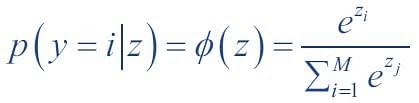
In probability theory, the output of the Softmax function represents a probability distribution over K different outcomes.
In Softmax, the probability of a particular sample with net input z belonging to the ith class can be computed with a normalization term in the denominator, that is, the sum of all M linear functions:
The Softmax function is used in ANNs and Naïve Bayes classifiers.
For example, if we take an input of [1,2,3,4,1,2,3], the Softmax of that is [0.024, 0.064, 0.175, 0.475, 0.024, 0.064, 0.175]. The output has most of its weight if the original input is '4’ This function is normally used for:
- Highlighting the largest values
- Suppressing values that are significantly below the maximum value.
The Softmax function is demonstrated here.
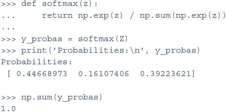
This code implements the softmax formula and prints the probability of belonging to one of the three classes. The sum of probabilities across all classes is 1.
Let us talk about Hyperbolic functions in the next section.
Hyperbolic Functions
1. Hyperbolic Tangent
Hyperbolic or tanh function is often used in neural networks as an activation function. It provides output between -1 and +1. This is an extension of logistic sigmoid; the difference is that output stretches between -1 and +1 here.
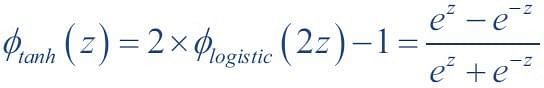
The advantage of the hyperbolic tangent over the logistic function is that it has a broader output spectrum and ranges in the open interval (-1, 1), which can improve the convergence of the backpropagation algorithm.
2. Hyperbolic Activation Functions
The graph below shows the curve of these activation functions:
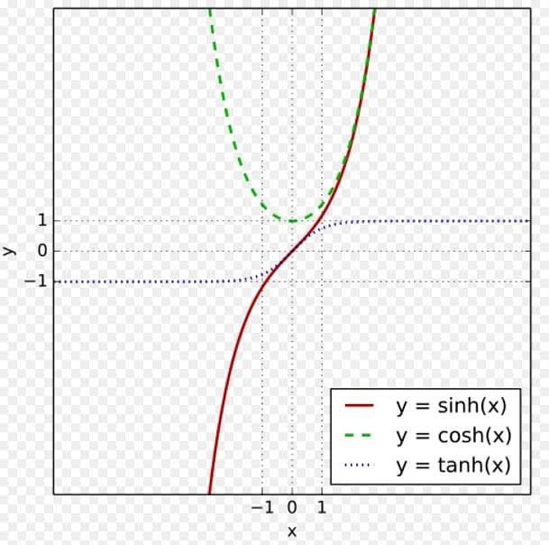
Apart from these, tanh, sinh, and cosh can also be used for activation function.

Based on the desired output, a data scientist can decide which of these activation functions need to be used in the Perceptron logic.
3. Hyperbolic Tangent
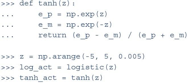
This code implements the tanh formula. Then it calls both logistic and tanh functions on the z value. The tanh function has two times larger output space than the logistic function.
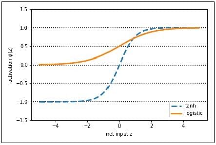
With larger output space and symmetry around zero, the tanh function leads to the more even handling of data, and it is easier to arrive at the global maxima in the loss function.
Are you curious to know what Deep Learning is all about? Watch our Course Preview to know more.
Activation Functions at a Glance
Various activation functions that can be used with Perceptron are shown below:
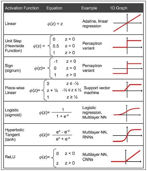
The activation function to be used is a subjective decision taken by the data scientist, based on the problem statement and the form of the desired results. If the learning process is slow or has vanishing or exploding gradients, the data scientist may try to change the activation function to see if these problems can be resolved.
Summary
Let us summarize what we have learned in this tutorial:
- An artificial neuron is a mathematical function conceived as a model of biological neurons, that is, a neural network.
- A Perceptron is a neural network unit that does certain computations to detect features or business intelligence in the input data. It is a function that maps its input “x,” which is multiplied by the learned weight coefficient, and generates an output value ”f(x).
- ”Perceptron Learning Rule states that the algorithm would automatically learn the optimal weight coefficients.
- Single layer Perceptrons can learn only linearly separable patterns.
- Multilayer Perceptron or feedforward neural network with two or more layers have the greater processing power and can process non-linear patterns as well.
- Perceptrons can implement Logic Gates like AND, OR, or XOR.
Comments
Post a Comment